Passive temperature sensors are the first choice in building control systems. They are cheap and easy to install thanks to their polarity independence, compared to active sensors with voltage or current output. However, deployment of passive sensor may lead to problems, which – and debugging of which – are dealt in the following article.
In the building control systems several types of passive temperature sensors can be found:
That is why the most commonly used sensor types in HVAC systems are these:
Both Ni1000 types are not fully compatible with each other, a look in the temperature-to-resistance table shows that even at room temperatures, the measuring difference is about 4 K, and more than 10 K at hot water. That is why attention must be paid when replacing old technologies with new controllers: it may seem that the value is OK because when commissioning, a simple I/O check may not reveal the problem.
When measuring resistance, the sensor is powered by a constant current source, and the voltage drop at the sensor is measured. The basic input circuit schematics (e.g. according to the Amit s.r.o. application note) is at Fig. 1. The circuit is usually enhanced by filters, surge protection elements etc.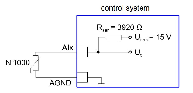
Fig. 1: Input circuit of an analogue input
The Ut voltage is brought into an A/D converter. Based on the voltage, the sensor resistance is calculated, and the result is linearized according to the conversion table resistance / temperature for the respective sensor type. It should be noticed that the controller measures not only the resistance of the sensor, but also that of the cable between the controller and the sensor, inclusive parasitic resistances of the terminals, connectors etc. This results in the first rule for the installation of passive sensors:
The sensor cable should be brought directly to the controler terminals, with no cable extensions, no input terminals in the panel, no common grounds for more sensors etc. The cable must have sufficient wire cross-section, minimum 2×0,8 mm2 is recommended. It is not advisable to use UTP cables. If the cable is longer than about 20 to 30 meters, the cable resistance should be calculated. Note that this is a 2 wire cable, and the total cable resistance is equal to nominal resistance of the wire * cable length * 2. If the measuring error plays a significant role (it reads about 1 K for every 4 Ohms for Pt1000), it should be noted in the project so that the programmer would introduce a software correction, or deployment of an active sensor should be considered.
A permanent measuring current in a sensor might lead to its excessive heating. This is why pulse measuring is used: the measuring current is multiplexed and brought into the sensor for e.g. 12.5 % of the total time, which coincides with the number of analogue inputs per one A/D converter in the controller, or even for a shorter time. This must be noted when checking the sensor with a multimeter which displays mean value only. The best tool is an oscilloscope, as will be shown later.
This is the most common type of problems. They are caused by mistakes in projects, and by bad quality installation. A galvanic influencing of measured value follow if the input circuits of the temperature-measuring controller are run through a parasitic current from other circuits. This current either flows through the controller input to common signal ground, or creates a voltage drop at the wiring from the sensor to the controller. This is typical if there is a common ground for passive and active sensors (water pressure, relative humidity, air quality etc.).
Fig. 1 shows a completely wrong wiring where the power supply current of the pressure sensor flows through the red conductor. The pressure sensor and mainly the temperature sensor are affected by the voltage drop which rises at the red-marked conductor. In fact, this means that the sensor shows higher value than the measured value, so the temperature sensor (or all sensors at the common A/D converter) show 149 °C or similar out-of-range value, depending on the maximum range of the input. Of course, this would influence the control algorithms, and the system indicates DHW overheating, high temperature at the heat exchanger etc.
 Fig. 2: Wrong wiring of a passive sensor
When trying to fix the problem as shown on Fig. 3, the sensor is connected using a 4-wire cable, and the power is brought over a separate pair G – G0. However, the temperature sensor is connected to a common ground (also known as signal ground) at the input terminals of the panel, at the point marked A at Fig. 3. The problem still persists: the voltage drop caused by the current flowing from the active sensor to the input is added to the sensor voltage which has to be measured with millivolt accuracy (in the input circuit as of Fig. 1, voltage of 12 mV represents about 1 K).
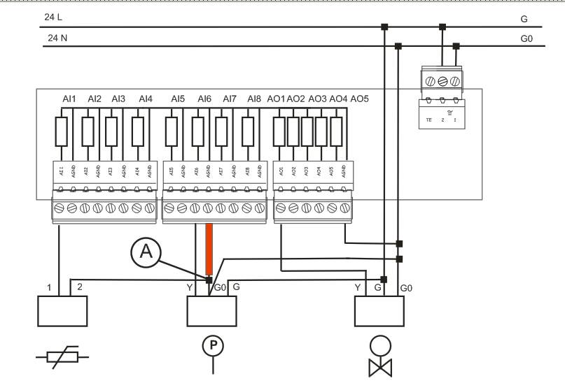 Fig. 3: Another wrong wiring of a passive sensor
Finally, wiring as of Fig. 4 should solve these problems.
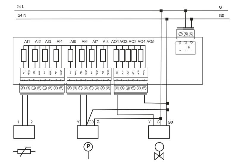
Fig. 4: Correct wiring of a passive sensor
Note, however, that Fig. 4 shows a loop between analogue output ground, G0, active sensor ground, analogue input ground and its connection to analogue output ground inside of the I/O module. This is where an AC voltage may be induced, which, again, influences the measured values. What could help here is separation of AI and AO grounds within the I/O module (which is mostly a module construction problem and little can be done about that), or at least bringing the G0 conductor of the active sensor as close to the I/O module as possible and then along the outputs to G0, so that the loop area is as small as possible.
At a project, a temperature sensor and a valve were wired as shown at Fig. 3. (The situation with active output peripherials, such as valves or dampers, is the same as with active sensors, if not worse because of their higher consumption.) As the water temperature decreased, the controller increased the voltage at the analogue output to open the valve, which resulted in temperature increase caused by parasitic voltage. The controller reacted accordingly, closed the valve a bit, the parasitic signal decreased, and the temperature seemed to drop down. The circuit stabilized after a while, keeping the proper „temperature“, unfortunately, too low in reality.
The problems related to grounding are numerous and it is not easy to get rid of them. The first point is that the shop drawings of the panel should be available. Note that the common potentials as G0, TE, N, PEN are plotted on a topological basis, i. e. the drawing usually does not specify from where and where the conductors are drawn, but only their connection which assumes zero resistance of the conductor.
In reality, the measuring is influenced by the resistance of the conductors, even inside of the panel. It is then necessary to use common terminal blocks and bars for all common potentials, like PE, N, G, G0, and connections between the peripherials, controller I/Os and other components should be pulled always to these bars and as short as possible. A good installation practice helps here especially for the second group of problems, which have a common determination: interference induced by AC current.
The induced interference is tricky as it propagates on a wireless basis. The induced voltage may origin from numerous sources. Usually, they are variable speed drives (VSD), photovoltaic inverters, switched power supplies or 3rd party systems as motors, industrial appliances or other devices.
The main focus in protection against induced interference is good-quality installation. The critical points are:
It says that a bad shielding is worse than no shielding. A poorly grounded shielding works, in fact, as a receiving antenna. The shielding conductors and strips should be connected in a single point which should be connected to earth (TE) or PEN by a copper wire with sufficient cross section, as close to the input terminals as possible. See Fig. 5. Separate screw terminals should be used, just twisting the wires into a single bunch is not enough. The shielding should be grounded at one end only (in the panel) to prevent loops. The other end is either left disconnected (and isolated), or connected to local ground over a ceramic capacitor of about 100 nF. It proved good to leave the other end disconnected, though.
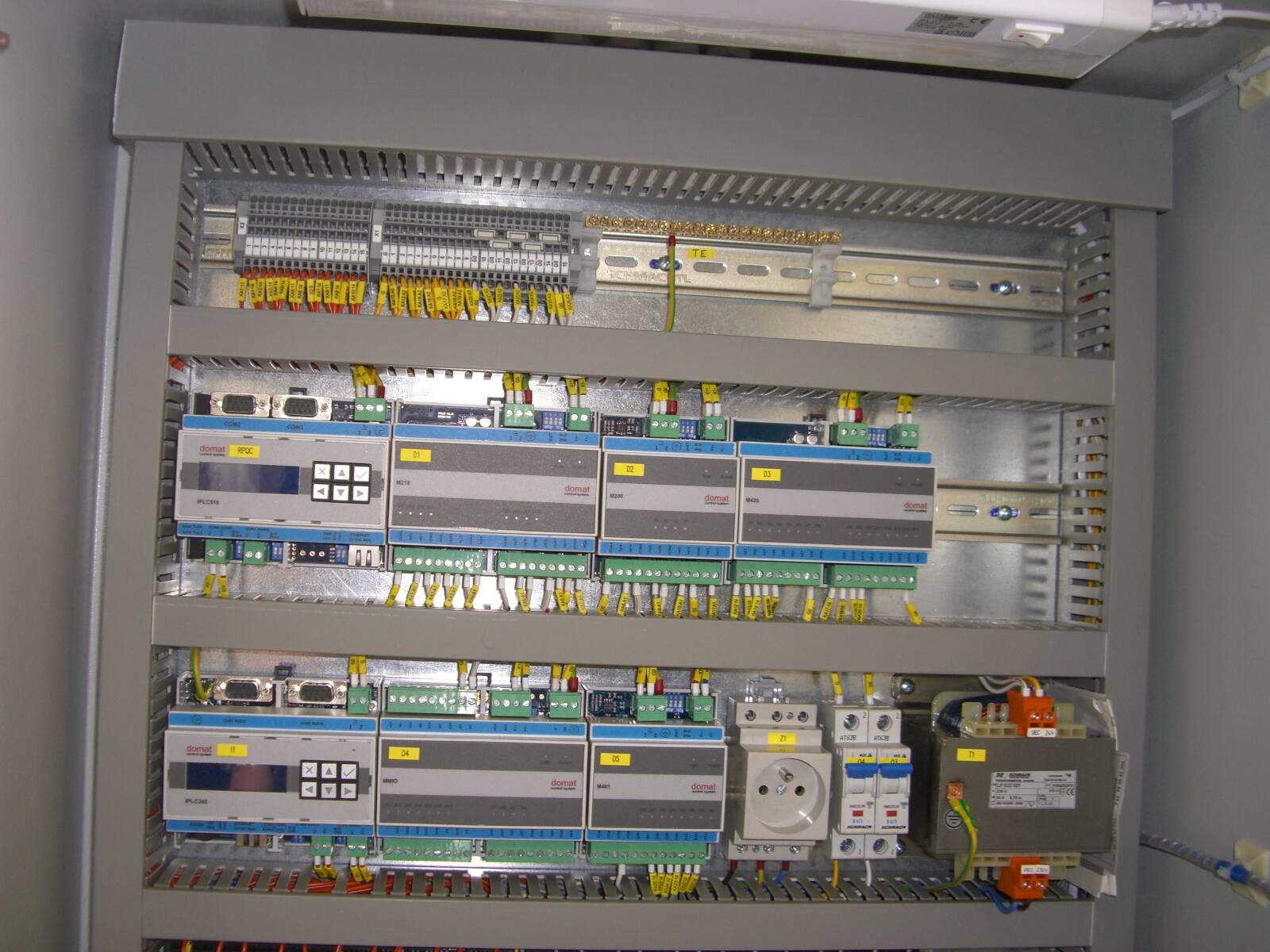 Fig. 5: In the upper part, close to the input terminals, there is the TE terminal block ready for connection of the shielding
The input circuits of the controllers are usually equipped with 50 or 60 Hz filters which should suppress the AC humming. However, filters may not be efficient against interferences coming from VSDs, switched power supplies, and PV inverters. Even worse news is that higher frequencies propagate better than 50 Hz grid frequency.
A good tool for diagnostics is an oscilloscope which shows not only presence of the disturbing signals but also frequency, shape and presence in time. This may help in locating the root of the signals. The proceedings are more or less as follows:
As soon as the measured temperatures „flow away“, look at the disturbing signal shape and magnitude (DC offset / 50 Hz / another frequency), check the proper connection of the peripherial which is at question and try to find why (in combination with already connected I/Os!) it is causing the measuring error. Usually, common grounds or parallel runs are located, it also helps to try to separate the power supply (add a separate 24 V supply). It is useful to have a spare power supply at hand, be it a cheap power adapter with 12 or 24 V output.
When using oscilloscope, note that the probe ground is usually connected with the protective earth. To be able to connect the probe ground to „our“ ground in the panel, a UPS must be used to power the oscilloscope. Disconnect the UPS from grid when measuring.
It is important how the I/O modules are designed, especially at combined modules (containing more signal types, such as AI and AO). Some examples here:
Note that at the modules with higher separation, AI and AO grounds must be connected if 3-wire active sensors are used together with analogue 3-wire output peripherials, so that the analogue signal is related to the common power and signal ground of the sensors and valves / actuators, namely G0.
It may also help to connect the 24 V AC ground (G0) to the shielding ground (Technical Earth, TE), which stems from the protective earth (PE nebo PEN). However, this is not a galvanically correct solution, because the 24 V AC system should be separated from the ground.
Software corrections may be accepted only as a compensation of the parasitic resistance of the cable. I saw an attempt once to introduce aa dynamic correction in case that the temperature seemed to increase when the VSD speed went higher. The programmer intended to change the software correction value dynamically in the program, based on the control signal for the VSD; this certainly is not the right attempt, it does not remove the cause, and may be used perhaps just as a temporary measure before the wiring and shielding are fixed, filters installed etc. (Unfortunately, this kind of hotfix usually lasts forever, and therefore solutions like this should be avoided.)
If the problem persists, it proved good to use a separate I/O module for the critical inputs or outputs (VSDs), where the output is galvanically totally separated from all the other I/Os, or – and this seems to be the ultimate solution – to use a galvanically separated communication line to control the VSD. This saves I/O points, and makes possible to integrate plenty of other signals including discrete and cumulated values, such as error codes, operating hours etc.
